1 Introduction

2 Introduction

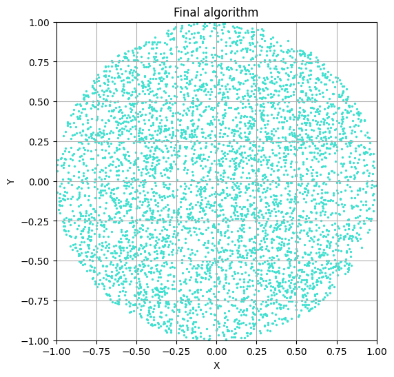
YouTube recommendations can sometimes lead to surprisingly insightful videos. One such example is the video The BEST Way to Find a Random Point in a Circle by nubDotDev, which was originally submitted to 3blue1brown’s Summer of Math Exposition. This video addresses an interesting problem: How would you write an algorithm to sample points uniformly within a circle?

Uniformly sampled points inside a circle

Before reading this post, I recommend watching the video, as it covers rejection sampling and polar coordinate methods to solve this problem. In the following sections, I will present another solution that neither relies on rejection sampling nor polar coordinates, but instead utilizes the equation of a circle directly. Why would you want to know about all this? I’m not sure, but maybe this simple problem stimulates your curiosity like it did for me, so I recommend doing it for this purpose alone.

Note

As already mentioned, there exist many solutions to this problem, like the rejection-sampling method. This post is about the result of my own ideas of thinking about the problem, but of course, these are not new and can be found in the existing approaches.

3 Uniform Sampling

3.1 Naive Approach

The equation for a circle of radius \(r\) centered at the origin is given by:

\[ y^2 + x^2 = r^2 \tag{1}\]

Using Equation 1, random points on a circle can be sampled by selecting random values for \(x \in [0,r]\) and calculating the corresponding \(y\) value (or vice versa). This only gives us points lying on the circle, whereas our objective is to sample uniformly from the entire area within the circle. This can be achieved by additionally sampling the radius as \(r_{\text{sampled}} \in [0,r]\). To summarize, the following procedure can be followed as our first attempt to sample points uniformly within a circle of radius \(r = 1\):

Sample \(r_{\text{sampled}} \in [0,1]\)
Sample \(x \in [0, r_{\text{sampled}}]\)
Calculate \(y\) (Equation 1)
Plot the point \((x,y)\)

To keep the code simple, we’ll just create a quarter circle, that is use \(x,y \in [0,1]\).

import matplotlib.pyplot as plt
import numpy as np

# Number of points to sample
num_points = 1000

# Arrays to store the sampled points
x_points = []
y_points = []

for _ in range(num_points):
    r = np.random.uniform(0, 1)
    x = np.random.uniform(0, r)
    y = np.sqrt(r**2 - x**2)
    x_points.append(x)
    y_points.append(y)

# Plotting the points
plt.figure(figsize=(6, 6))
plt.scatter(x_points, y_points, color='turquoise', s=2)
plt.xlim(0, 1)
plt.ylim(0, 1)
plt.xlabel('X')
plt.ylabel('Y')
plt.title('Initial Sampling - Points Clustered Around Center')
plt.grid(True)
plt.show()

3.2 Circumference sampling

This method is simple, but it has a couple of problems, resulting in a non-uniform density of points. The most obvious problem is, that the points are denser around the circles’ center. The problem arises because the circumference of the circle grows with \(r_{\text{sampled}}\) but the number of samples \(k\) doesn’t, as shown in this image.

As the circumference grows, the number of samples remains the same, resulting in a non-uniform density of samples.

To fix this, we can simply generate more points as the circle grows. Specifically, we’ll use the circumference \(c\) as a scaling factor.

\[ c = 2 \pi r_{\text{sampled}} \tag{2}\]

def points_based_on_circumference(r, scale=1):
    return int(np.ceil(2 * np.pi * r * scale))

x_points = []
y_points = []
num_radii = 1000

for _ in range(num_radii):
    r = np.random.uniform(0, 1)
    num_points = points_based_on_circumference(r)
    for _ in range(num_points):
        x = np.random.uniform(0, r)
        y = np.sqrt(r**2 - x**2)
        x_points.append(x)
        y_points.append(y)

plt.figure(figsize=(6, 6))
plt.scatter(x_points, y_points, color='turquoise', s=2)
plt.xlim(0, 1)
plt.ylim(0, 1)
plt.xlabel('X')
plt.ylabel('Y')
plt.title('Improved Distribution with Circumference-Based Sampling')
plt.grid(True)
plt.show()

3.3 Inverse

Now we notice the second problem: It seems like there are fewer points at the bottom of the diagram. To explain what’s going on, it’s easier to look at a single circle generated with this approach.

Code

# Number of points to sample
num_points = 100

# Arrays to store the sampled points
x_points = []
y_points = []

for _ in range(num_points):
    # Sample r from [0, 1]
    r = 1

    # Sample x from [0, r]
    x = np.random.uniform(0, r)

    # Calculate y based on the circle formula X^2 + Y^2 = r^2
    y = np.sqrt(r**2 - x**2)


    # Append the point to the arrays
    x_points.append(x)
    y_points.append(y)

# Create the plot
plt.figure(figsize=(6, 6))
plt.scatter(x_points, y_points, color='turquoise', s=5)

# Set the limits and labels
plt.xlim(0, 1)
plt.ylim(0, 1)
plt.xlabel('X')
plt.ylabel('Y')
plt.title('Points on a Circle')
plt.grid(True)

# Show the plot
plt.show()

Because the circle is drawn by calculating \(y\) via \(x\), which is uniformly sampled, there are simply more values on the “roof” of the circle than on the side, because from the perspective of \(x\), the area is wider. We can fix t his problem by also considering the perspective of \(y\), that is inverting \(x\) and \(y\) by chance.

import random

# Number of points to sample
num_points = 100

# Arrays to store the sampled points
x_points = []
y_points = []

for _ in range(num_points):
    # Sample r from [0, 1]
    r = 1

    if random.random() < 0.5:
      # Sample x from [0, r]
      x = np.random.uniform(0, r)

      # Calculate y based on the circle formula X^2 + Y^2 = r^2
      y = np.sqrt(r**2 - x**2)
    else:
      y = np.random.uniform(0, r)
      x = np.sqrt(r**2 - y**2)


    # Append the point to the arrays
    x_points.append(x)
    y_points.append(y)

# Create the plot
plt.figure(figsize=(6, 6))
plt.scatter(x_points, y_points, color='turquoise', s=5)

# Set the limits and labels
plt.xlim(0, 1)
plt.ylim(0, 1)
plt.xlabel('X')
plt.ylabel('Y')
plt.title('Points on a Circle')
plt.grid(True)

# Show the plot
plt.show()

3.4 Full circle

Using the \(c\) as a factor for the number of samples \(k\) and by inversing \(x\) and \(y\) by chance, we can finally generate a full circle. This is done by sampling \(x \in [-r_{\text{sampled}}, r_{\text{sampled}}]\) and mirroring the point on the x-axis by chance.

import matplotlib.pyplot as plt
import numpy as np

# Function to determine the number of points based on the circumference
def points_based_on_circumference(r, scale=1):
    return int(np.ceil(2 * np.pi * r * scale))

# Arrays to store the sampled points
x_points = []
y_points = []

# Number of different radii to sample
num_radii = 1000

for _ in range(num_radii):
    # Sample r from [0, 1]
    r = np.random.uniform(0, 1)

    # Number of points to sample for this radius
    num_points = points_based_on_circumference(r)

    for _ in range(num_points):
        if random.random() < 0.5:
          # Sample x from [0, r]
          x = np.random.uniform(-r, r)

          # Calculate y based on the circle formula X^2 + Y^2 = r^2
          y = np.sqrt(r**2 - x**2)
          if np.random.rand() > 0.5:
            y = -y
        else:
          y = np.random.uniform(-r, r)
          x = np.sqrt(r**2 - y**2)

          if np.random.rand() > 0.5:
            x = -x

        # Randomly decide the sign of y to cover both the top and bottom halves


        # Append the point to the arrays
        x_points.append(x)
        y_points.append(y)

# Create the plot
plt.figure(figsize=(6, 6))
plt.scatter(x_points, y_points, color='turquoise', s=2)

# Set the limits and labels
plt.xlim(-1, 1)
plt.ylim(-1, 1)
plt.xlabel('X')
plt.ylabel('Y')
plt.title('Points on Circles with Different Radii')
plt.grid(True)

# Show the plot
plt.show()

With a bit more refactoring, we can also make the code more compact and reusable.

Refactored code

import matplotlib.pyplot as plt
import numpy as np
import math

target_r = 10

r_granularity = 500
c_granularity = 1

# Function to determine the number of points based on the circumference
def points_based_on_circumference(r, granularity):
    return int(np.ceil(2 * np.pi * r * granularity))

# Arrays to store the sampled points
x_points = []
y_points = []

# Number of different radii to sample
for _ in range(r_granularity):
    r = np.random.uniform(0, target_r)

    # Number of points to sample for this radius
    num_points = points_based_on_circumference(r, c_granularity)

    for _ in range(num_points):
        # Sample and calculate vars
        dep = np.random.uniform(-r, r)
        indep = np.sqrt(r**2 - dep**2)

        # Mirror on x-axis
        if np.random.rand() > 0.5:
          indep = -indep

        # Assign indep. and dep. var
        x, y = (dep, indep) if np.random.rand() > 0.5 else (indep, dep)

        # Append the point to the arrays
        x_points.append(x)
        y_points.append(y)

3.5 Blurring the lines

However, with this approach, we will encounter a final problem. For small values of r_granularity, it becomes clear that the points are sampled on separate circles.

Code

target_r = 10

r_granularity = 25
c_granularity = 5

# Function to determine the number of points based on the circumference
def points_based_on_circumference(r, granularity):
    return int(np.ceil(2 * np.pi * r * granularity))

# Arrays to store the sampled points
x_points = []
y_points = []

# Number of different radii to sample
for _ in range(r_granularity):
    r = np.random.uniform(0, target_r)

    # Number of points to sample for this radius
    num_points = points_based_on_circumference(r, c_granularity)

    for _ in range(num_points):
        # Sample and calculate vars
        dep = np.random.uniform(-r, r)
        indep = np.sqrt(r**2 - dep**2)

        # Mirror on x-axis
        if np.random.rand() > 0.5:
          indep = -indep

        # Assign indep. and dep. var
        x, y = (dep, indep) if np.random.rand() > 0.5 else (indep, dep)

        # Append the point to the arrays
        x_points.append(x)
        y_points.append(y)

# Create the plot
plt.figure(figsize=(6, 6))
plt.scatter(x_points, y_points, color='turquoise', s=2)

# Set the limits and labels
plt.xlim(-target_r, target_r)
plt.ylim(-target_r, target_r)
plt.xlabel('X')
plt.ylabel('Y')
plt.title('target_r = 10, r_granularity = 25, c_granularity = 5')
plt.grid(True)

# Show the plot
plt.show()

To solve this problem, we can replace the scaling factor, which is calculated using the circumference \(c\) with a probability. So instead of deterministically drawing \(k = c_{\text{sampled}} = 2 \pi r_{\text{sampled}}\) points on a circle with radius \(r_{\text{sampled}}\) we will only draw one point with probability \(p = \frac{c_{\text{sampled}}}{c}\).

target_r = 1

r_granularity = target_r * 10000

# Function to determine the number of points based on the circumference
def p_acc_based_on_circumference(r):
    return (2 * np.pi * r) / (2 * np.pi * target_r)

# Arrays to store the sampled points
x_points = []
y_points = []

# Number of different radii to sample
for _ in range(r_granularity):
    r = np.random.uniform(0, target_r)

    # Number of points to sample for this radius
    p_acc = p_acc_based_on_circumference(r)

    if np.random.rand() < p_acc:
        # Sample and calculate vars
        dep = np.random.uniform(-r, r)
        indep = np.sqrt(r**2 - dep**2)

        # Mirror on x-axis
        if np.random.rand() > 0.5:
          indep = -indep

        # Assign indep. and dep. var
        x, y = (dep, indep) if np.random.rand() > 0.5 else (indep, dep)

        # Append the point to the arrays
        x_points.append(x)
        y_points.append(y)

# Create the plot
plt.figure(figsize=(6, 6))
plt.scatter(x_points, y_points, color='turquoise', s=2)

# Set the limits and labels
plt.xlim(-target_r, target_r)
plt.ylim(-target_r, target_r)
plt.xlabel('X')
plt.ylabel('Y')
plt.title('Final algorithm')
plt.grid(True)

# Show the plot
plt.show()

4 Extra

The approach introduced in the previous sections works not only for circles but also for other shapes. The different components like Equation 1 or the ways of mirroring can be adjusted to create entirely new shapes with uniformly sampled points. I will leave it up to the reader to find the changes made to each of these following shapes, resulting in this variety.

Code

import matplotlib.pyplot as plt
import numpy as np

# Function to determine the number of points based on the circumference
def points_based_on_circumference(r, scale=100):
    return int(np.ceil(2 * np.pi * r * scale))

# Arrays to store the sampled points
x_points = []
y_points = []

# Number of different radii to sample
num_radii = 1000

for _ in range(num_radii):
    # Sample r from [0, 1]
    r = np.random.uniform(0, 1)

    # Number of points to sample for this radius
    num_points = points_based_on_circumference(r) // 20

    for _ in range(num_points):
        # Sample x from [-r, r]
        x = np.random.uniform(-r, r)

        # Calculate y based on the circle formula X^2 + Y^2 = r^2
        y = np.sqrt(r - x**2)

        # Randomly decide the sign of y to cover both the top and bottom halves
        if np.random.rand() > 0.5:
            y = -y

        # Append the point to the arrays
        x_points.append(x)
        y_points.append(y)

# Create the plot
plt.figure(figsize=(6, 6))
plt.scatter(x_points, y_points, color='firebrick', s=2)

# Set the limits and labels
plt.xlim(-1, 1)
plt.ylim(-1, 1)
plt.xlabel('X')
plt.ylabel('Y')
plt.title('Modified shape 1')
plt.grid(True)

# Show the plot
plt.show()

Code

import matplotlib.pyplot as plt
import numpy as np

# Function to determine the number of points based on the circumference
def points_based_on_circumference(r, scale=100):
    return int(np.ceil(2 * np.pi * r * scale))

# Arrays to store the sampled points
x_points = []
y_points = []

# Number of different radii to sample
num_radii = 1000

for _ in range(num_radii):
    # Sample r from [0, 1]
    r = np.random.uniform(0, 1)

    # Number of points to sample for this radius
    num_points = points_based_on_circumference(r) // 20

    for _ in range(num_points):
        # Sample x from [-r, r]
        x = np.random.uniform(-r, r)

        # Calculate y based on the modified equation X + Y = r
        y = r - abs(x)

        # Randomly decide the sign of y to cover both the top and bottom halves
        if np.random.rand() > 0.5:
            y = -y

        # Append the point to the arrays
        x_points.append(x)
        y_points.append(y)

# Create the plot
plt.figure(figsize=(6, 6))
plt.scatter(x_points, y_points, color='firebrick', s=2)

# Set the limits and labels
plt.xlim(-1, 1)
plt.ylim(-1, 1)
plt.xlabel('X')
plt.ylabel('Y')
plt.title('Modified shape 2')
plt.grid(True)

# Show the plot
plt.show()

Code

import matplotlib.pyplot as plt
import numpy as np

# Function to determine the number of points based on the circumference
def points_based_on_circumference(r, scale=100):
    return int(np.ceil(2 * np.pi * r * scale))

# Arrays to store the sampled points
x_points = []
y_points = []

# Number of different radii to sample
num_radii = 5000

for _ in range(num_radii):
    # Sample r from [0, 1]
    r = np.random.uniform(0, 1)

    # Number of points to sample for this radius
    num_points = points_based_on_circumference(r) // 100

    for _ in range(num_points):
        # Sample x from [-r, r]
        x = np.random.uniform(-r, r)

        # Calculate y based on the equation x + y = r
        y = r - abs(x)

        # Randomly decide the sign of y to cover both the top and bottom halves
        if np.random.rand() > 0.5:
            y = -y

        # Append the point to the arrays
        x_points.append(x)
        y_points.append(y)

# Create the plot
plt.figure(figsize=(6, 6))
plt.scatter(x_points, y_points, color='firebrick', s=2)

# Set the limits and labels
plt.xlim(-1, 1)
plt.ylim(-1, 1)
plt.xlabel('X')
plt.ylabel('Y')
plt.title('Modified shape 3')
plt.grid(True)

# Show the plot
plt.show()